A graph of actions
All the steps in a simulation are encapsulated in actions. The basic action types can be a change to an input deck, running an OpenFOAM analysis, or extracting results from an analysis.
Some actions are used for control e.g. to set up the simulation as a graph where some actions depend on other actions.
The diagram below illustrates a workflow where a single geometry creation step leads to two parallel analysis branches: one for OpenRadioss and another for LS-DYNA. Each branch includes meshing and parameterization steps, and finally, the results from both solvers are combined to compute the overall design performance.
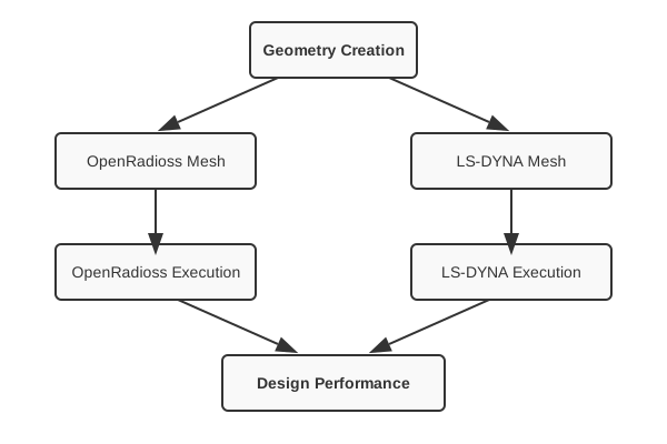
Actions
An action defines an operation in the workflow. It can be anything from a geometry creation, an FEA analysis, to mathematical computations. Once you have an action defined, you can call the ‘solve()’ method to execute.
The input to ‘solve()’ method, supplied by the user, is
a dictionary containing the variable values;
for example, {'var_A': 3.1, 'var_B': 7 }.
The input to a lower level ‘solve()’ method, supplied by the graph, is
a dictionary containing
the variable values supplied to the toplevel ‘solve()’ call together
with the outputs of the previous actions in the graph;
for example, {'var_A': 3.1, 'var_B': 7, 'action_Z': array([2, 1, 2])}.
The return value of the ‘solve()’ method depends on the action; for example, for a d3plot database extraction it may return the extracted data as a numpy array.
You can call the ‘solve()’ method on a graph. In which case it will return a dictionary
containing the names and return values of all the children;
e.g. {'child_A': array([2, 1, 2]), 'child_B': 3.1}.
A child that is itself a graph — a sub-graph, a WorkArea, or a
d3plot_File, which is a workflow of extractions — contributes its own
dictionary under its name rather than merging its results into the
parent’s, so its values are reached as ret['child_graph']['value'].
from kunene.dyna_actions import DynaAnalysis
dyna = DynaAnalysis(name="RunSpring", input_path="spring.k")
ret = dyna.solve( {'K': 100.} )
You can chain actions to edit a mesh or extract results as described below.
User actions
You can create your own action by subclassing WorkAction
and defining the action in the ‘solve()’ method.
The optional description argument documents what the action returns.
If omitted, the class docstring is used.
See the previous section for a description of the solve method.
from kunene.actions import WorkAction

class AdderAction(WorkAction):
    """Adds two numbers and returns the sum."""
    def solve(self, val_dict=None):
        a = val_dict.get('a', 0)
        b = val_dict.get('b', 0)
        return a + b

# With an explicit description:
adder = AdderAction(name='add', description='Sum of inputs a and b')
Setting up a graph
Two types of graphs are available: firstly, a WorkFlow, a simple version executing the actions sequentially; and a DirectedGraph, which allows execution to branch and execute actions in parallel.
To use a WorkFlow to evaluate actions sequentially:
from kunene.d3plot_actions import d3plot_File
from kunene.dyna_actions import DynaAnalysis
from kunene.graph_actions import WorkFlow

wf = WorkFlow(name="SpringWorkFlow")
wf.add_action( DynaAnalysis(name="RunSpring", input_path="spring.k") )
d3p = d3plot_File( name='d3p' )
d3p.NodalValue(name='n5', state=1, nid=5, component= 'node_displacement'  )
wf.add_action( d3p )

ret = wf.solve( {'K': 100.} )

# 'd3p' is itself a graph, so its extractions sit under its name
print( 'Displacement of node 5', ret['d3p']['n5'] )
To use a DirectedGraph. The example below runs the same spring deck through two solvers and compares the answers — an OpenRadioss branch and an LS-DYNA branch that execute independently, and a merge action that waits for both:
from kunene.actions import MathEvaluation
from kunene.d3plot_actions import d3plot_File
from kunene.dyna_actions import DynaAnalysis
from kunene.graph_actions import DirectedGraph, WorkFlow, WorkArea
from kunene.radioss_using_dyna_inp import RadiossUsingDynaInput

dg = DirectedGraph( name='MDO', asynch=True )

# OpenRadioss branch: the LS-DYNA deck run by OpenRadioss
rad_wf = WorkFlow( name='RadiossBranch' )
rad_wf.add_action( RadiossUsingDynaInput( name='rad',
                                          cmd='rad_dyna_inp',
                                          input_path='spring.k',
                                          create_d3plot=True ) )
rad_d3p = d3plot_File( name='d3p' )
rad_d3p.NodalValue( name='rad_n5', state=1, nid=5, component='node_displacement' )
rad_wf.add_action( rad_d3p )

rr = dg.add_action( WorkArea( rad_wf, copy_paths=['path/to/spring.k'] ) )

# LS-DYNA branch
dyna_wf = WorkFlow( name='DynaBranch' )
dyna_wf.add_action( DynaAnalysis( name='RunSpring', input_path='spring.k' ) )
dyna_d3p = d3plot_File( name='dyna_field' )
dyna_d3p.NodalValue( name='dyna_n5', state=1, nid=5, component='node_displacement' )
dyna_wf.add_action( dyna_d3p )

rs = dg.add_action( WorkArea( dyna_wf, copy_paths=['path/to/spring.k'] ) )

# Merge back: runs once both branches have finished
dg.add_action( MathEvaluation( name='solver_diff',
                               cmd='abs( rad_n5 - dyna_n5 )' ),
               parents=[ rr, rs ] )

ret = dg.solve( {'K': 100.} )

print( 'Solver difference at node 5', ret['solver_diff'] )
Three things in that example are worth spelling out.
Each branch gets its own directory. Both solvers write a d3plot
file, and both would write it into the current directory, so each branch
is wrapped in a WorkArea. add_action returns the action it was
given, so the returned work areas are what the merge action names as its
parents. See Work areas and design studies.
Results stay structured. A WorkArea contributes its outputs as a
nested dictionary under its own name, and so does the d3plot_File
inside it — which is what keeps two branches with similar action names
apart. Each level also carries the values that were passed into it:
{ 'K': 100.0,
  'RadiossBranch_WorkArea': {
      'K': 100.0,
      'rad': True,                     # the solver reported normal termination
      'd3p': { 'K': 100.0, 'rad': True,
                     'rad_n5': array([40.127, 0., 0.]) } },
  'DynaBranch_WorkArea': {
      'K': 100.0,
      'RunSpring': True,
      'dyna_field': { 'K': 100.0, 'RunSpring': True,
                      'dyna_n5': array([40.127, 0., 0.]) } },
  'solver_diff': array([0., 0., 0.]) }
A MathEvaluation flattens this view before evaluating, so its
expression refers to rad_n5 and dyna_n5 directly, without naming
the work area or the d3plot reader they sit in. Note that
node_displacement is a three-component vector, so solver_diff is
an array rather than a single number.
The two solvers run at the same time. asynch=True starts
independent actions — here the two solver work areas — in separate
processes, so the design takes about as long as its slower solver rather
than the sum of the two. The merge action still waits for both, because
it was added with parents=[rr, rs]. Leave asynch out to run the
solvers one after the other. The children run in the graph’s own working
directory, which is the other reason the solvers have a WorkArea each.
Running in parallel covers what else follows from the solvers running in
separate processes, and how to run the designs of a study in parallel
as well.
Call dg.describe_workflow() to print the action tree and the
directory structure the run will create, without running anything or
having the solvers installed.